Almost all low cost MEMS gyroscope outputs are contaminated with additive sinusoidal noises. However, these additive sinusoidals are hindered by the additive white noise (ARW) most of the time. Therefore, these components are usually missed in the inertial sensor models by the inexperienced engineers (the experienced ones also usually miss it, but I prefer to call those as ignorant stupids rather than engineer).
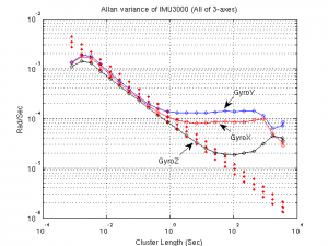
Here is an example. The following is the Allan variance of the IMU3000:
It looks quite normal, doesn’t it?
Well then. Let’s play with it a little bit by downsampling the GyroY data as follows:
- gdat5=GyroY(1:5:end);
- gdat10=GyroY(1:10:end);
- gdat15=GyroY(1:15:end);
- gdat20=GyroY(1:20:end);
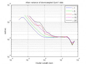
Just the simple downsampling. And now, let’s compute the allan variance of each of these downsampled data. In the following figure, you can see the computed Allan variances for the downsampled version of the GyroY (together with the original one).
What a striking result we have! The Allan variance of the gdat10, gdat15 and gdat20 (red, magenta and black curves) have a very strange additional bulge on their initial segments. Where do they come from? What happened?
Let me explain what you have just witnessed. When we downsample the data, we change the frequency of the additive sinusoidal error (remember the effect of downsampling operation on sine/cosine functions). The downsampling shifted the frequency of these sinuosidal components to the lower part of the signal spectrum where the Allan variance coefficients are computed with a smaller frequency window (in other words with a larger time window/cluster). The power of the white noise within that smaller window is obviously less. As the windows get smaller, the power of the additive noise becomes smaller than the power of sinusoidal components. From that point on, we can start seeing the effect of sinusoidal components on the Allan variance figures. But of course this procedure is also upper limited. For very large cluster lengths (narrow frequency windows) the sine function is also filtered out.
As you can see from the figure above, IMU3000 has a serious additive sinusoidal noise problem. An inexperienced navigation engineer can easily miss this fact if he/she just trusts simple Allan variance figures (because, the ignorant stupids usually advices them to do so).
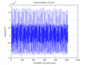
In fact, one should always use correlation based analysis techniques together with the Allan variance figures in order not to miss such important error components. As an example, you can see the correlation of the GyroY output in the following figure.
The figure speaks for itself. We can immediately see that the correlation is a sinusoidal function.
To tell the truth, I first computed this correlation only to observe that we have an additive sinusoidal component problem for this sensor. And then, I came up with this downsampling idea in order to be able to see it in the Allan variance figures. (Yes, it is my original invention. But feel free to use it whenever you want to annoy stupid ignorants.)
Unfortunately, the autocorrelation computation for the inertial sensors is not simple. If you just try to compute the autocorrelation with “xcorr” function (of matlab), you won’t be able to see anything other than a triangular waveform. One should subtract the “approximate” signal before computing the autocorrelation. (The modelling section of the toolkit should give you some idea about how to do it properly.) However, as this example suggests, the results that we obtain is usually worth the additional efforts that we spent for correlation computation.


